04 · Spatial analysis (squidpy-GPU)

Mirrors the rapids-singlecell squidpy tutorial. metal-SingleCell’s msc.gr namespace is a drop-in for squidpy.gr, GPU-accelerated on Apple silicon. We use squidpy’s IMC (imaging mass cytometry) dataset — it has cell-type labels and channel intensities, so we can show spatial autocorrelation and the fused-kernel co-occurrence analysis.

import warnings; warnings.filterwarnings('ignore')
import numpy as np, scanpy as sc, squidpy as sq
import metalsinglecell as msc

adata = sq.datasets.imc()
adata

AnnData object with n_obs × n_vars = 4668 × 34
    obs: 'cell type'
    uns: 'cell type_colors'
    obsm: 'spatial'

Spatial neighbors graph

Builds obsp['spatial_connectivities'] from obsm['spatial'].

msc.gr.spatial_neighbors(adata, n_neighs=6)
adata.obsp['spatial_connectivities'].shape

(4668, 4668)

Moran’s I — global spatial autocorrelation

Which channels vary smoothly across the tissue?

msc.gr.spatial_autocorr(adata, mode='moran', genes=adata.var_names.tolist(), n_perms=100)
adata.uns['moranI'].head(8)

	I	pval_sim
3521227Gd155Di Slug	0.770918	0.009901
6967Gd160Di CD44	0.528501	0.009901
1031747Er167Di ECadhe	0.473841	0.009901
234832Lu175Di panCyto	0.463043	0.009901
971099Nd144Di Cytoker	0.412303	0.009901
phospho mTOR	0.411461	0.009901
346876Sm147Di Keratin	0.396131	0.009901
98922Yb174Di Cytoker	0.393929	0.009901

Geary’s C — a complementary autocorrelation statistic

msc.gr.spatial_autocorr(adata, mode='geary', genes=adata.var_names.tolist(), n_perms=100)
adata.uns['gearyC'].head(8)

	C	pval_sim
92964Er166Di Carboni	1.040275	0.702970
117792Dy163Di GATA3	0.988649	0.534653
Area	0.929862	0.009901
8001752Sm152Di CD3epsi	0.925628	0.425743
phospho S6	0.919657	0.069307
322787Nd150Di cMyc	0.895445	0.346535
378871Yb172Di vWF	0.861285	0.009901
1441101Er168Di Ki67	0.853448	0.009901

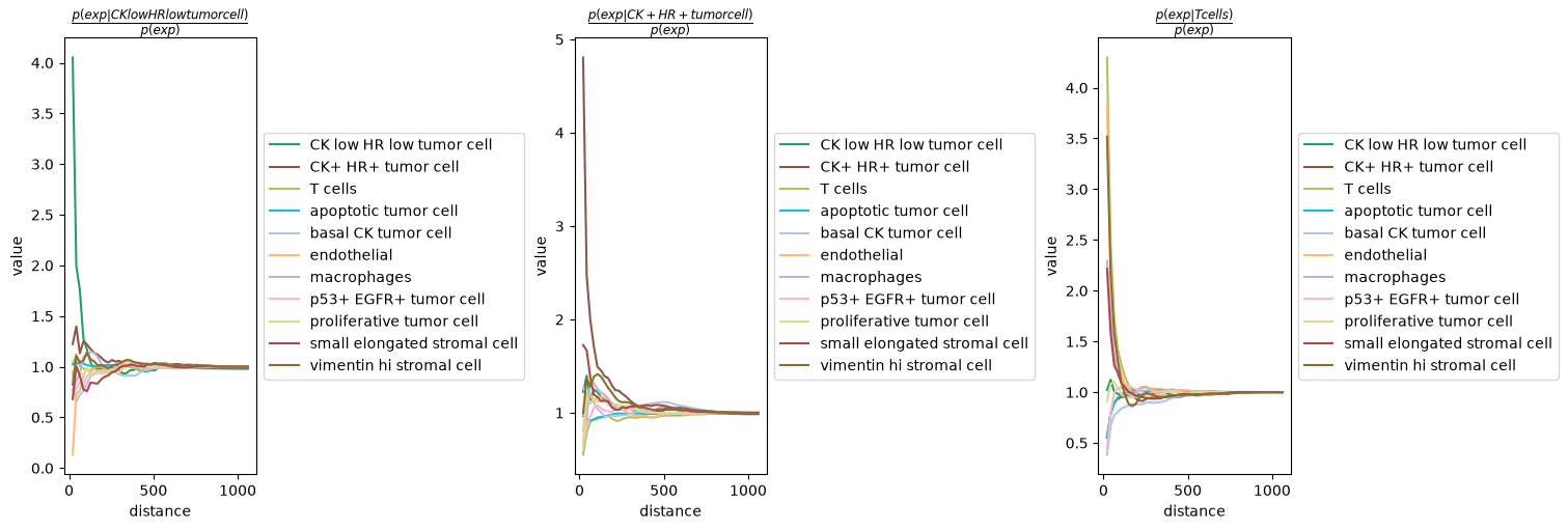
Co-occurrence — how cell types cluster vs distance

co_occurrence uses a fused Metal atomic-histogram kernel (tiled, scales to large sections). It measures the enrichment of each cell type around a target type as a function of radius.

msc.gr.co_occurrence(adata, cluster_key='cell type', interval=50)
occ = adata.uns['cell type_co_occurrence']['occ']
print('co-occurrence tensor (types × types × radii):', occ.shape)

co-occurrence tensor (types × types × radii): (11, 11, 50)

try:
    sq.pl.co_occurrence(adata, cluster_key='cell type',
                        clusters=list(adata.obs['cell type'].cat.categories[:3]))
except Exception as e:
    print('squidpy plot skipped:', e)

Visualize the tissue

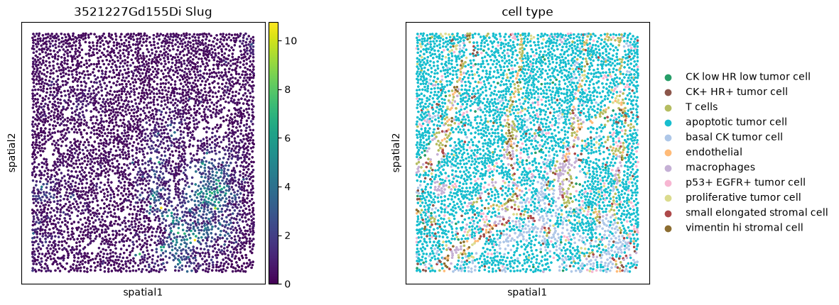
Top spatially-autocorrelated channel and the cell-type map.

top_gene = adata.uns['moranI'].index[0]
sq.pl.spatial_scatter(adata, color=[top_gene, 'cell type'], shape=None, size=8)

WARNING: Please specify a valid `library_id` or set it permanently in `adata.uns['spatial']`

All spatial graph statistics (spatial_neighbors, spatial_autocorr for Moran/Geary, co_occurrence) ran on the Apple GPU and match squidpy’s CPU results exactly.